

Our not-so-magic journey scaling low latency, multi-region services on AWS
Engineering stateless, high-availability cloud services comes with juuuuuuust a few challenges. Here’s how we (eventually) slayed the dragon.
Atlassian went “all in” on AWS in 2016 and they continue to be our preferred cloud provider. The extent of that migration was covered from a high-level in this article. But what we didn’t cover in that piece was the number of services we needed to modify or build to be stateless.
I’d like to tell you the tale of one of these new services, which would serve as the central point of the transition – a context service which needed to be called multiple times per user request, with incredibly low latency, and be globally distributed. Essentially, it would need to service tens of thousands of requests per second and be highly resilient as downtime could result in a cloud-wide loss of functionality for Atlassian.
Let me explain all of our optimizations, in chronological order, in order to meet (and exceed!) the heavy requirements placed on this context service. I hope that it offers good architectural patterns others can use when building similar services.
The architectural problem
When trying to build stateless services you quickly run into a problem – try as you might, something actually has to care about state. In the simplest case, you would offload that to the database with some sort of partition key that is allocated to each customer (internally referred to as a “tenant”). This approach works fine for basic use cases, but let’s consider a more complex example, Jira, and its requirements:
- In order to reduce the blast radius, noisy neighbour problems and enable horizontal scaling, we decided to create smallish groups of tenants.
- These tenant groups (“shards”) were globally distributed.
- Jira’s existing non-AWS infrastructure operated on a DB-per-tenant model. It was not feasible for us to change this model as part of our migration to AWS. Thus, each Jira instance still used a unique DB, although we did have multiple DBs on a single RDS instance.
Consider now a (heavily simplified) example of a request to a Jira instance “foo.atlassian.net”:
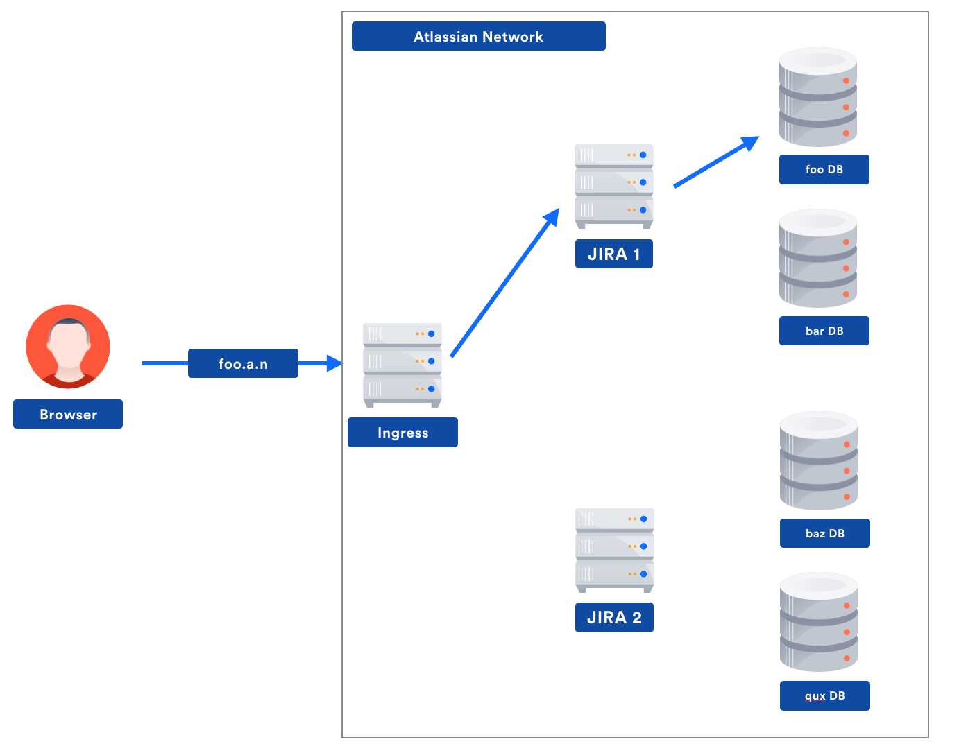
In this example, there are two distinct decision points where “which tenant is issuing the request?” is relevant:
- Our network ingress service needs to know which Jira shard to talk to in order to reduce latency for the customer.
- Jira needs to know which DB has the tenant’s data.
Therefore, we either need both ingress and Jira to maintain a global mapping of tenants to the right shard / DB or, even better, we need to centralise this knowledge with a singular service that maintains the required tenant → location mapping. The service would store a piece of context and look vaguely like:
{
  "jira": {
     "db-user": "kurashiki",
     "db-password": "jumpydoll"
  },
  "network-ingress": {
    "/": "http://jira-us-east-1.aws.stack"
    "/wiki": "http://confluence-eu-west-2.aws.stack"
  },
  ... <Other tenant metadata, e.g. active products, license counts, other product info>
}
In practice, this service actually ends up being used for a lot more than just routing Jira calls, acting more like a generalised tenant metadata service, or say, a Tenant Context Service (TCS) across all of Atlassian cloud.
It also gives us pretty clear requirements on the service. It needs to:
- Support extremely numbers of requests per second at the lowest possible latency (as it’s called multiple times per request to any Atlassian cloud service)
- Be globally distributed in all Atlassian Cloud regions
- Have 4-5 9s of availability
- Ensure that context data is never permanently corruptible
- Ensure that context data can be access controlled to only show the relevant pieces to each consumer for each product (e.g., no Confluence DB creds for Jira)
- Support a typical access pattern of key-value lookups (data is logically separated between tenants)
These requirements, or at least similar styles of requirements, are probably familiar to anyone who has had to write a datastore service of some variety. In our case, the latency and uptime guarantees were particularly aggressive – if TCS is down, then no requests to the customer’s instance can succeed. Generally, this is referred to as a non-desired state both internally and by our customers.
The first cut: CQRS with DynamoDB
Any eagle-eyed reader would notice that a lot of the requirements above can be met by simply using a high performant noSQL store. We had the same realization and decided to build on top of DynamoDB – which promises single digit response times, 5 9s of availability, and is available in many locations around the world – instead of trying to do it ourselves.
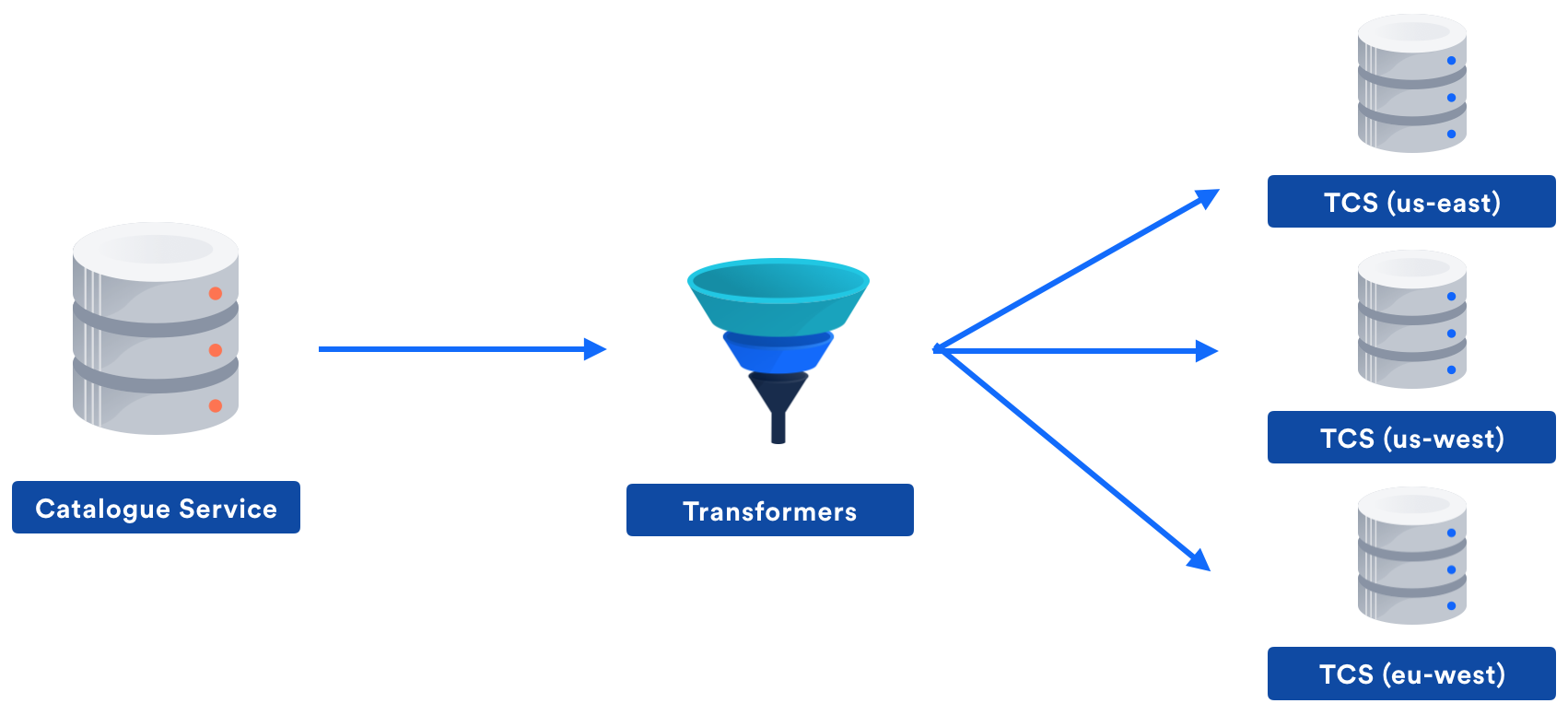
As part of this work, we employed a CQRS pattern. This provided one service to handle the source of truth data and deal with updates (Catalogue Service). Catalogue Service would then send the records to another service via AWS Kinesis in order to map these records to each individual use case. The resulting denormalized records were fed into another Kinesis stream and processed by logically independent TCS deployments in multiple regions.
This approach gave some very nice properties:
- Catalogue Service could enforce strong consistency without affecting TCS read performance.
- Catalogue Service had uptime and latency requirements that were an order of magnitude easier compared to TCS.
- “Multi-region” would only involve deploying TCS in many regions and reading from the same input stream.
- Each use case could output its own context data, which allows for data isolation between use cases and less network bandwidth used.
- We can optimise TCS to be a highly performant read-only store.
- Clients calling TCS can have failover logic, if a region is down, they can simply swap to using a backup region with no availability penalty.
Thus, we went about building this system. To be honest, it performed really well overall, especially in the early stages as we migrated customers over to the new stateless platform. Unfortunately, as we migrated more load over, the cracks started to show…
Lesson 1: DynamoDB is not magic
DynamoDB is great for many things, including our use case, but is not a silver bullet for fixing all of your data storage problems. As we scaled up load to a few thousand requests per second per region we started to notice some interesting patterns in our service performance and availability:
- Sometimes an entire AZ would get 5xx responses from DynamoDB for about 1 second, which was usually followed by it happening in a different AZ a few minutes later.
- Some requests would return extremely slowly (10+ ms) from DynamoDB and so we were unable to meet our response time objectives at the higher percentiles.
It’s worth noting that this is not saying DynamoDB was a bad choice, or that it wasn’t meeting SLAs. It remained the best choice of data store for our simple key-value data, and all failed requests or long response times were strictly within SLAs. Additionally, we had no immediate visibility into if the response times were due to DynamoDB itself, or things like connection establishment. The failures could also have been due to DNS being flakey (or being updated) as opposed to DynamoDB.
Regardless, it was a problem we needed to fix and we explored two main approaches:
- Optimise calls to DynamoDB (look into DNS, connection establishment, DynamoDB itself).
- Don’t call DynamoDB for every request.
You’ll note that option two is simply to cache. This means it has the best chance of fully fixing the problem, but would likely result in even lower response times from the service and saves us a bunch of money from just not calling DynamoDB as much.
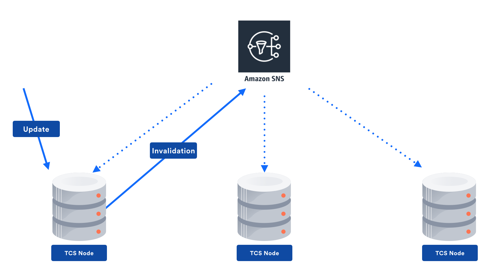
We also were thinking about adding a distributed cache like DynamoDB Accelerator (DAX), Redis or Memcached, but remember that TCS’s biggest focus is on read performance. Due to this, we were very keen to try and avoid all network calls on as many requests as possible. In order to do this, we’d need node-local caching. Additionally, while eventual consistency is great, downstream services generally get a little annoyed if eventual ends up meaning “a very very long time.” Therefore, an invalidation mechanism is still needed.
We started experimenting with sending the invalidations between nodes by using Amazon SNS:
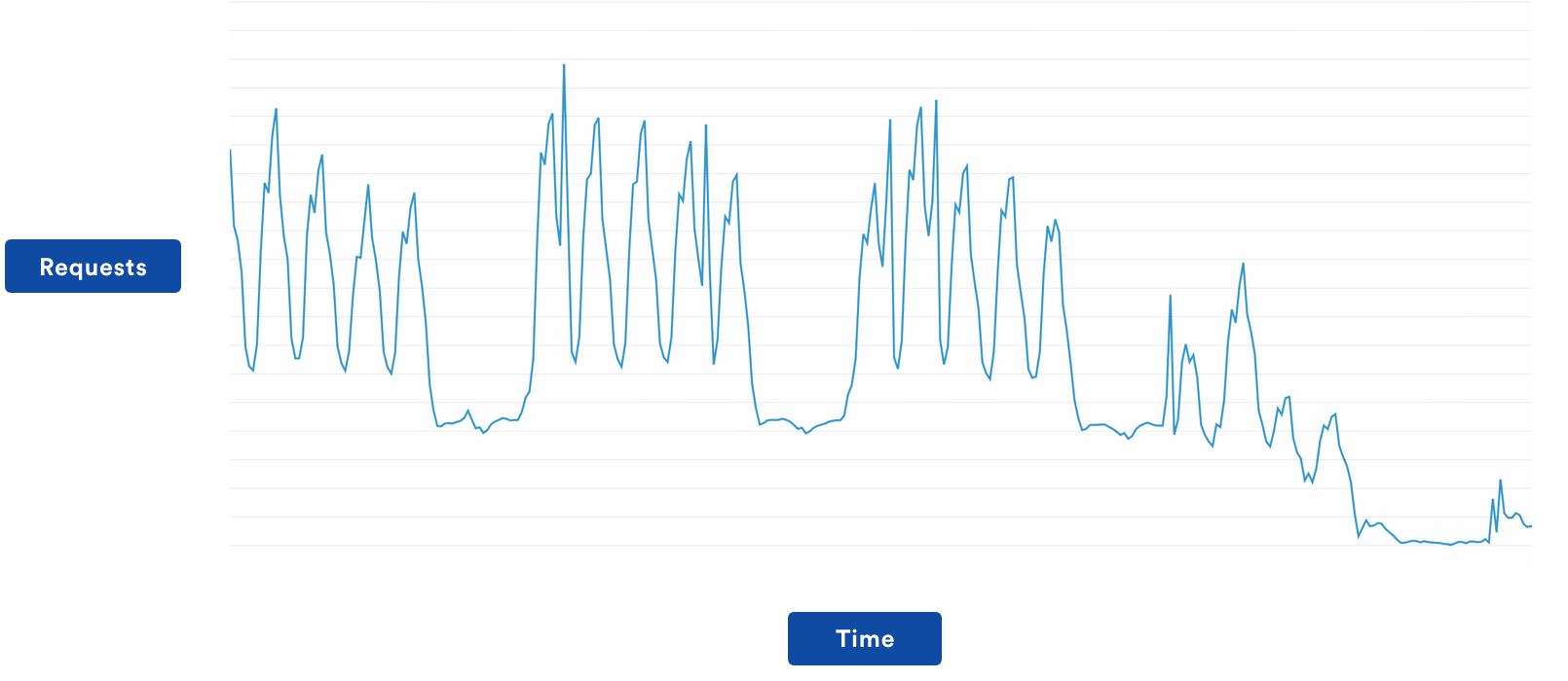
This resulted in invalidations taking a bit longer than if we used a distributed cache, but read performance massively increased. The drastic change is best illustrated through the following graphs, which are not aggregate, but particular TCS regions. I’ll leave it to the reader to figure out when the caching change went live!
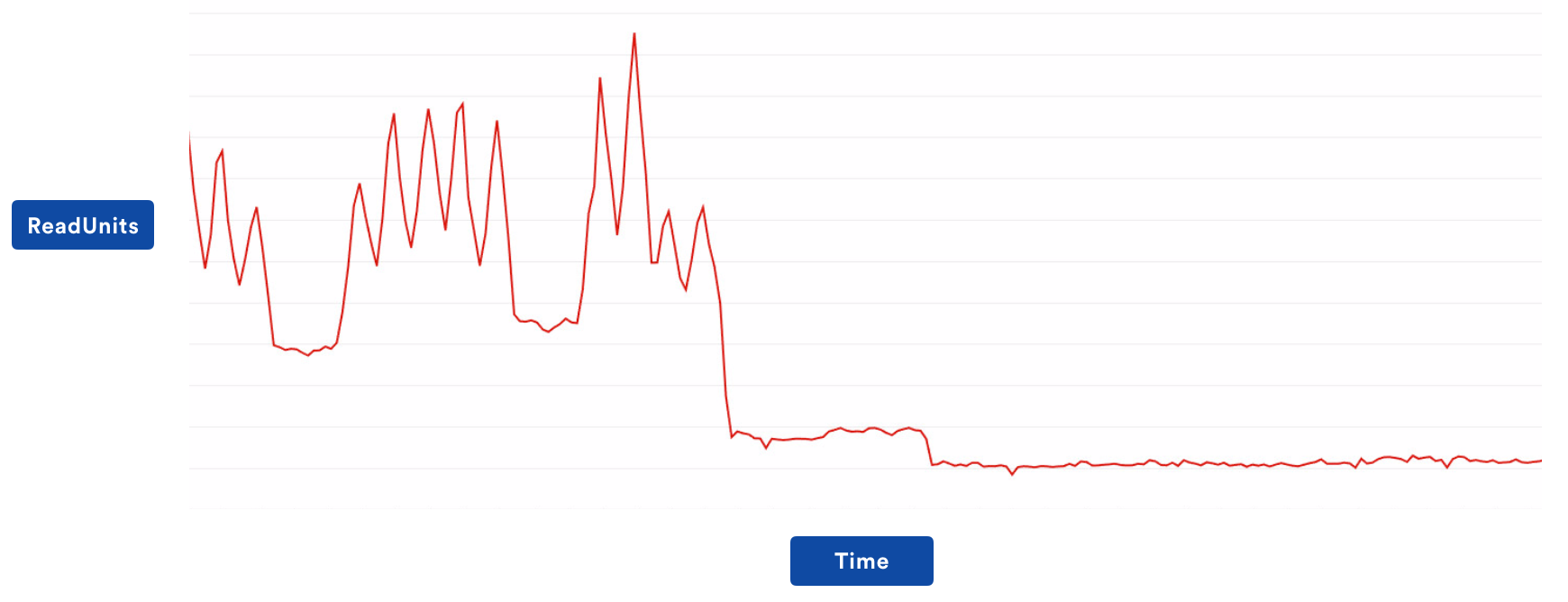
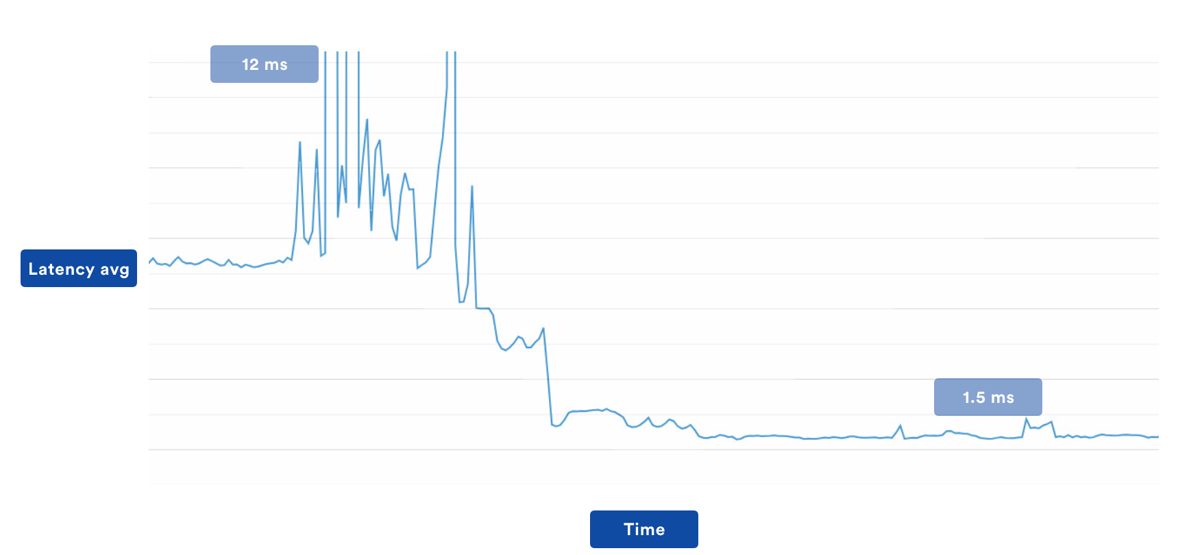
This simple change was all it took to enable us to migrate all customer load over to the new stateless architecture. For a couple of months, we didn’t have to touch it at all, but it wasn’t the end of the story. Which brings me to my next point…
Lesson 2: Load balancers are not magic
Much to our surprise, TCS had a brief outage in two U.S. regions for about five minutes. This was not good. A five-minute outage for two regions meant that all our cloud products were down for those five minutes in the U.S. (other regions were fine).
First, we looked at our metrics. Nothing stood out in particular for service monitoring, except this weird graph for requests against our Elastic Load Balancer (ELB).
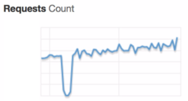
First, we looked at our metrics. Nothing stood out in particular for service monitoring, except this weird graph for requests against our Elastic Load Balancer (ELB).
For the period of the outage we didn’t fail, we just got zero requests to the ELB. Clearly, something was wrong, but based on all available metrics we couldn’t determine what specifically. Somewhat at a loss, we contacted AWS support and asked if they had any better metrics on their side. Thankfully they did and, as it turns out, the ELBs had died due to out of memory errors. The period of ‘zero requests’ that we were seeing in our metrics was simply due to the fact that there was no available ELB to service the requests. Everything recovered fine once a new ELB was scaled up.
At first glance, this seems like maybe the ELBs were faulty. But much like DynamoDB, the ELBs were actually operating within SLA – TCS just need to perform above that. Of note, ELBs have the following scaling characteristic: the time required for Elastic Load Balancing to scale can range from 1 to 7 minutes.
When TCS failed, it was immediately after a new stack deployment, where we replaced an old (scaled) ELB with a new one. The reason this happened was due to how our internal deployment process works, where it will bring up the new stack including the ELB as part of the deployment, then swap the DNS to point to the new ELB. This new ELB wasn’t scaled up to handle the traffic and thus died.
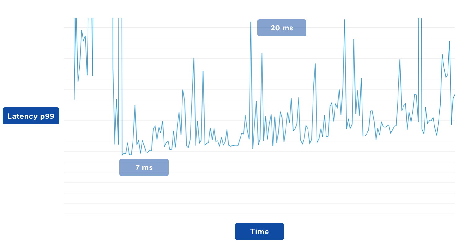
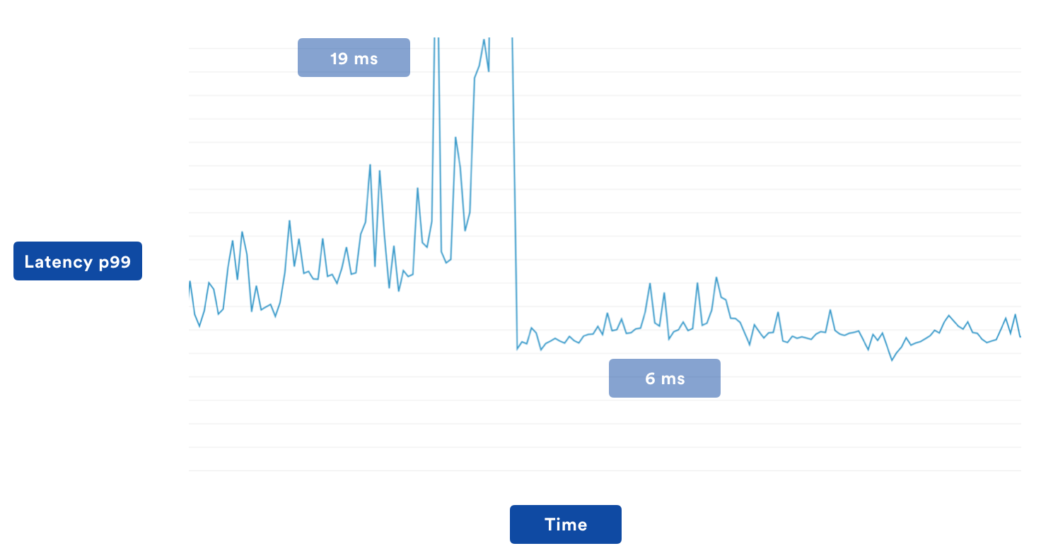
To fix the problem, we simply swapped to a single Application Load Balancer (ALB), since ALBs do not get cycled by our internal deployment process. This worked out great for reliability, and we’ve not had a similar outage since the switch. It did, however, have a rather unexpected side effect: our latency worsened for p99s, going from about ~7-10ms up to 20ms.
As it turns out, ELBs and ALBs actually use different routing algorithms. ELBs use “least connection first”, which sends requests to the webserver with the least open connections. ALBs use “strict round robin“ and send requests equally to all nodes.
This didn’t explain the bad p99 though even for the p99 case. A lot of the time we should be hitting the cache, or at the very worst doing a normal lookup to DynamoDB. At this point, our code was pretty streamlined, apart from language frameworks, the read path pretty much just read the cache, and on miss talked to DynamoDB…
Lesson 3: Caches are not magic
As it turns out, caches are not magic black boxes that always do what you expect. When we introduced the cache way back at the beginning of our optimisation journey, we decided to go with a Java Guava cache. We figured that it was widely used inside and outside the company already, supported by Google and was had a pretty simple API. This is still all true. However, Guava caches (and in fact many caches) have some interesting properties:
- Cache maintenance amortisation: Guava caches amortise maintenance such that every request does a little bit of maintenance, which results in no one request being saddled with it all.
- Going cold after a TTL: the cache has a TTL, after which time you have to go back to DynamoDB.
- No concurrent request throttling: if key X is requested by five callers at once and it’s a miss, you’ll end up with five calls to your backing store.
Now, these properties are all fine in the general case. It’s a really good general-purpose cache. However, it turns out that, as of Java 8, there’s a new, shinier cache built upon the foundation of Guava caches: Caffeine. Caffeine fixes all of our concerns with Guava caches, it adds background refresh, a dedicated maintenance executor and will block on concurrent stale requests.
We decided to test it out by doing a simple drop-in replacement for our guava cache:
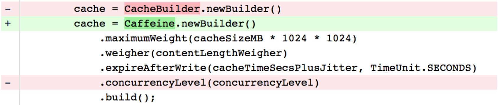
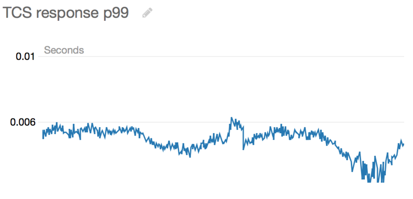
Finding when it was deployed to production should be pretty easy:
We then went ahead and further leveraged the extra features we had available, which proved to drastically improve both p99 response time (as above), while also giving decent benefits to the general case.
Lesson 4: Clients are not magic
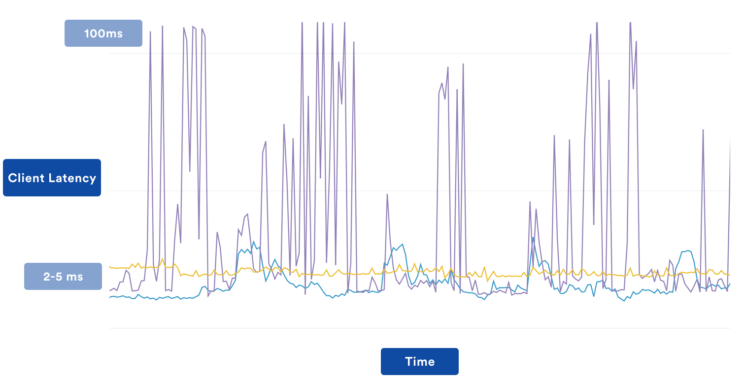
At this point, the TCS service itself was pretty rock solid – it was fast, reliable, and quiet. However, from time to time we had to particular internal teams complaining consistently that TCS was slow or failing. When we looked into it, we came up with the following chart, which reflects the average latency for calling TCS, as perceived from the client (this includes network time, as well as JWT token generation, which takes 1-3ms on average).
Take a guess at which team was complaining about TCS being slow.
We also cross-referenced the p99 metrics, which was still consistently below 6ms.
So, why was the average so high for one of our internal teams?
After some investigation, we found that the service in question was simplify not configured optimally to call TCS. Amongst other things, it was using sequential region calls, it had Guava caches with contention, and its HTTP connection pool was frequently exhausted. None of this is a knock on the developers of that service. As it turns out, writing super robust multi-region callable clients is hard, and when most of your job is actually focused on shipping customers useful features, you don’t always have the necessary time to invest in fine-tuning a bespoke client.
However, our team totally did have that time, and better, we could solve it for every service at once. Our solution was that we could write a small client sidecar that would run alongside any client who wished to talk to TCS. A sidecar is essentially just another containerised application that is run alongside the main application on the EC2 node. The benefit of using sidecars (as opposed to libraries) is that it’s technology agnostic – we could write our sidecar in whatever language we pleased and have it interop will all internal services. The service would then just need to make a localhost HTTP call and then our client would handle all the troublesome parts.
There were three main focuses for our client sidecar:
- Long-lived caches: not going on the network at all is always the fastest approach.
- Parallel multi-region requests: calling one region, then sequentially calling another if the first call fails is far too slow. We could write our client to call multiple regions at the same time and short-circuit whichever response came back first.
- Easy adoption: the API should be exactly the same as calling the “real” TCS.
Achieving #2 and #3 was easy enough. We achieved #1 by leveraging our existing SNS based cache invalidation logic. Instead of just having the main TCS webservers listening to the invalidation messages, now the clients were as well. Due to this, we could set the cache time to be upwards of an hour, while still getting only low single-digit seconds of update propagation time (which was actually better than the existing client’s “cache for 30 seconds unconditionally” behaviour).
To test it, we started by deploying it to a service that was already doing pretty well.
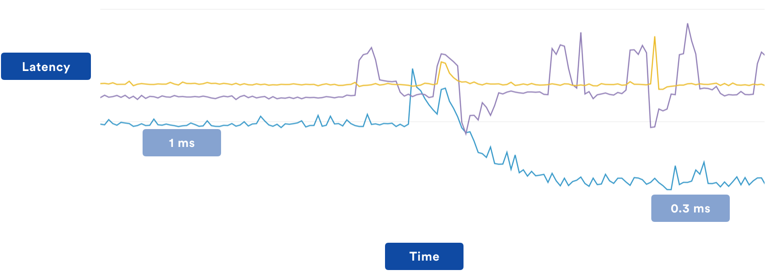
Given the positive response (as seen in the chart), we then deployed it to as many services as we could. As expected, latencies fell drastically. Interestingly though, requests to the main TCS service also fell drastically, even with the clients now sending requests to multiple regions in parallel, due to the significantly cleverer caching strategy.
Our current state
Since we started building TCS, we’ve onboarded more and more services to use it. All of the requirements we had for it before we started continue to be thoroughly exceeded. In short:
- Since introducing the client sidecar, we’ve seen almost 100% reliability. The only requests that “fail” are cases such as the entire client node disconnecting from DNS, or the node randomly dying (which as a sidecar we have no control over).
- p99 latencies from the client perspective are around ~0.7ms.
- We are not experiencing any client load problems, with more services being onboarded every quarter.
- There has been no source of truth data corruption or clients accessing other clients data.
Additionally, we had some fun putting it to the test via production chaos. We built the following automations that could be used on-demand:
- The ability to turn off entire regions
- Adding huge latency penalties for random requests
- Stopped regions from ingesting new records or ingesting them with significant delay
The best part? We could do all of these operations without any noticeable client impact.
What you should remember
- Isolating context/state management association to a single point is very helpful. This was reinforced at Re:Invent 2018 where a remarkably high amount of sessions had a slide of “then we have service X which manages tenant → state routing and mapping”. So it’s not just Atlassian.
- CQRS is seriously good. By isolating out concerns and clearly defining which use cases you want to optimise for, it becomes possible to invest the effort in the most mission-critical services without having to drag along other functionality at the same time.
- AWS is great. But it’s a foundation, not a solution. Do use AWS resources because they simplify service code so much. However, don’t fall into the trap of assuming that just because you used “the cloud” every problem will vanish. They just get replaced with different, higher level problems.
- Consider writing your own clients. As a service developer, you probably know how your service should be called in order to get the best performance. Make that easy for others to adopt. It could be via a library, a sidecar, or some other exotic way, but it’ll result in far fewer headaches for you and anyone who interacts with your service.
P.S. Our engineering teams are hiring. A lot. Just sayin’.