

Continuous profiling of JVM
Atlassian’s mission is to unleash the potential in every team. Our products help teams organize, discuss, and complete their work. Atlassian offers products and services such as Jira, Confluence, Trello, and Bitbucket. The products we build at Atlassian have hundreds of developers working on them, composed of a mixture of monolithic applications and microservices.
When an incident occurs in production, it can be hard to diagnose the root cause due to the high rate of change within the codebases. It is noticeably nontrivial to triage and reduce the impact radius of an incident to the most relevant contributing cause(s).
We always pursue techniques and tools that enable our engineers to apply performance engineering in their context, such as to diagnose a service at production. Profiling can speed up root-cause diagnosis significantly and is an effective technique to identify runtime hot spots and latency contributors within an application. Without profiling, it’s commonly necessary to implement custom and ad-hoc latency instrumentation of the code, which can be error-prone or cause other side effects. In addition, profiling allows exploration of unknowns at runtime whereas instrumentation requires planned work prior to runtime.
Profiling of JVM at Runtime
One of the frequently asked questions in many a diagnosis is (in one form or another):
What was the JVM doing during a particular time (from T1 to T2)?
When an incident occurs or an investigation kicks off, one of the first steps is to collect observations and facts of the running system. For a running JVM, there are well-established tools that allow us to look into JVM runtime around the process, threads’ state, memory, IO, and others.
In addition, profiling a JVM provides a precise way to understand the running code (via stack frames) in a JVM. There is also a well-established set of tools for profiling a JVM, for example, Visual VM.
One of the efficient tools to answer this question for JVM is a flame graph. A flame graph is a visualization of the running code inside a process that helps identify the most frequent code paths (for example, Java stack traces) in an accurate way.
The Journey of Profiling Tools
We started our journey to evolve our tooling for profiling JVM applications a few years ago. Like many other projects at Atlassian, the first step and building block completed was an innovation iteration, a practice that is greatly nurtured at Atlassian.
Initially, the goal was to create a simple tool, for example, a CLI for an engineer to be able to profile a running JVM at runtime in production and visualize the results as a flame graph.
To develop the tool, the following elements were implemented:
- A client to run a secure and safe shell script via AWS Systems Manager
- Bundled set of shell scripts approved by our platform to execute specific OS commands
- A bundled Linux perf and async-profiler next to running JVM applications
- HTTP clients to interact with storage systems such as AWS S3 to collect and provide the output
This was a great first success; i.e. an engineer was able to run a CLI to profile the target JVM application at runtime in production and capture the profiling data and visualize them using Flame Graphs.
We continued to develop the tool and expand its functions and usage across our teams. While the tooling was highly valuable, our method had some limitations:
- Intervention from a person (or system) was required to capture a profile at the right time, which meant transient problems were often missed. When an incident occurred, it was not deterministic when would be a good moment to trigger the tool to capture profiling data. In addition, layers of abstraction between the local CLI tool and the eventual shell scripts being executed added delays which could lead to missing the opportunity to capture the profiling data at the right time.
- Ad-hoc profiling didn’t provide a baseline profile to compare with. The profiling tools were only used by a manual run from an engineer and this mostly occurred during incidents. The captured profiling data for a single system were not unified to create a baseline.
- For security and reliability, a limited number of people had access to run these tools in production. Since the profiling tooling used shell script to run Linux command with elevated privileges, by security standards it was not open to all engineers across teams.
These limitations led us to look into continuous profiling; i.e., run the profiling tools on a set of target JVM applications based on a timed schedule and store the profiling data. There have been interesting challenges and trade-offs to build a reliable and efficient solution for continuous profiling:
- Runtime Overhead. Profiling a JVM at runtime is not without a cost, although there have been great efforts to build tools with minimal overhead. Continuous profiling adds to this overhead based on the schedule and frequency which might affect the performance of the system. The continuous profiling system needs to provide a balance between the overhead at runtime and the frequency of the profiling. The former decreases the performance of the JVM and the latter increases the efficiency of the captured profile data. The trade-off also depends on the load of the system at runtime.
- Accuracy of Profiling Data. The frequency of profiling directly influences its accuracy. The more frequently a profile is captured, the closer and smaller time windows the profiling data are available for analysis. This would allow the analysis of the system in arbitrary time windows with the possibility of aggregations. If profiling occurs infrequently or with a schedule, the captured profiling data would not be reliable for all the different investigational purposes; it’s mostly useful for a high-level view of the system.
- Storage and Retrieval of Profiling Data. The captured profiling data of a JVM does not have a small size, that is, order of few megabytes, for a 1,000-deep stack frame. The storage for such data is required to provide both short-term and long-term capabilities. For the short-term, fast retrieval is necessary to be able to drive quick investigations. For the longer term, aggregation and retention pose a new challenge.
We started to build an in-house continuous profiling solution. We decided to continue to use Linux perf and async-profiler, which came with several advantages, including:
- Data in a format that we could visualize as a flame graph (which is easy to interpret)
- The ability to profile either a single process or a whole node
- Profiling across different dimensions such as CPU, memory, and IO
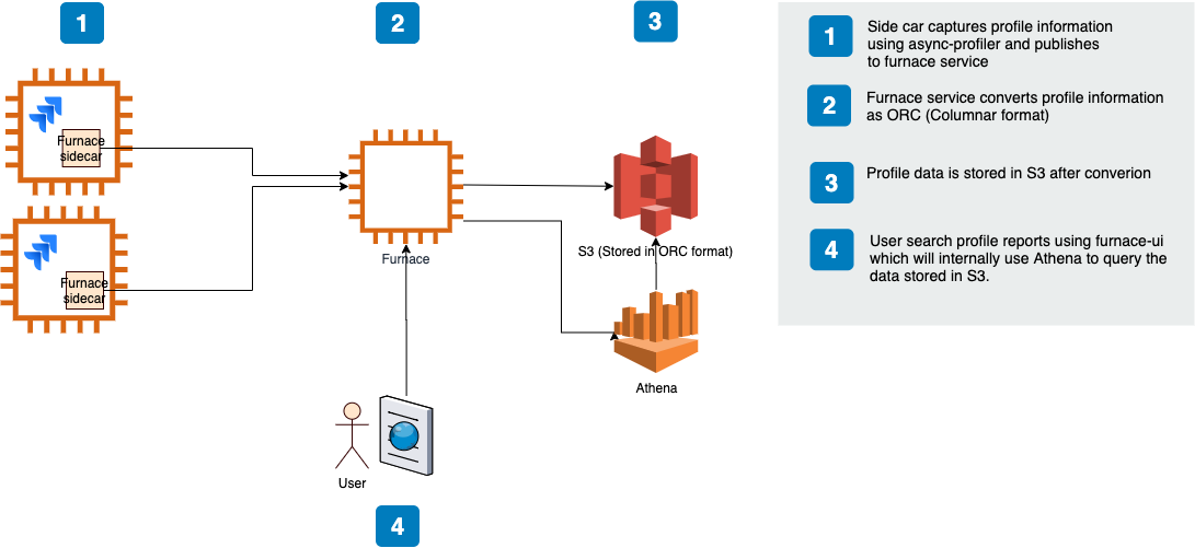
Our initial continuous profiling solution comprised
- a scheduled job that ran async-profiler (or Linux perf) regularly
- uploaded the raw results to a microservice that transformed the raw data into a columnar data format; Apache ORC. We also evaluated Apache Parquet but chose ORC mainly because of cost and efficiency of complex query executions
- and wrote the result to AWS S3
We defined a schema in AWS Glue allowing developers to query the profile data for a particular service using AWS Athena. Athena empowered developers to write complex SQL queries to filter profile data on dimensions like time range and stack frames. We also started building a UI to run the Athena queries and render the results as flame graphs using SpeedScope.

Adopting Amazon CodeGuru Profiler
Meanwhile, the announcement of Amazon CodeGuru Profiler caught our attention — the service offering was highly relevant to us and largely overlapped with our existing capability.
We foster an agile culture in our engineering practices at Atlassian. The ultimate goal was to bring the value of continuous profiling as a performance engineering tool to every engineer across development teams. We drove a spike to evaluate and experiment with Amazon CodeGuru Profiler. The results looked promising in terms of integration, capturing the data and analysis via visualization. Though, we also learned there are some limitations to this service in contrast with Linux perf or async-profiler. A few of those differences and limitations are as follows:
- Some features from async-profiler (or
perf_event API) are really interesting and useful, for example, lock profiling, the support of native stacks, and inlined methods. - The safe-point poll bias is a known issue with many JVM profilers including Amazon CodeGuru Profiler which does not exist in Linux perf nor async-profiler.
Even with the effort we already employed for our in-house solution, we still had significant work ahead of us to build out a user-friendly one in comparison with Amazon CodeGuru Profiler. The team needed to make a decision; continue our solution development or adopt Amazon CodeGuru Profiler. We made a balanced trade-off to switch to adopting Amazon CodeGuru Profiler.
We have now integrated Amazon CodeGuru Profiler at a platform level, enabling any Atlassian service team to easily take advantage of this capability.
Using continuous profiling for Latency in JVM Thread States. One of the first ways we utilized CodeGuru Profiler was to identify code paths that show obvious or well-known problems in terms of CPU utilization or latency. We searched for different forms of synchronization in the profiled data. For example, we searched for methods containing synchronized sub-string. Another useful feature of Amazon CodeGuru is that it provides a HotSpot view, in which the user can see the most frequent code paths also categorized by thread states. Therefore, we chose a random (relatively small) time frame and used the HotSpot view to find any BLOCKED thread state.
One interesting case was an EnumMap that was wrapped in a Collections.synchronizedMap. The following screenshot shows the thread states of the stack frames in this code path for a span of 24 hours.
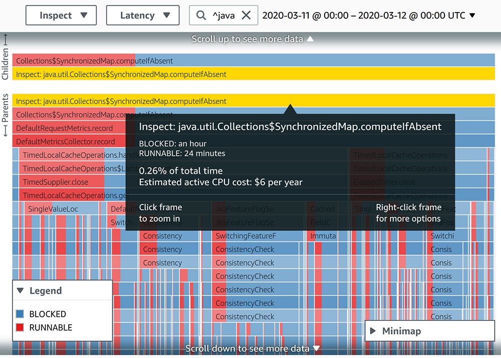
Although the involved stack trace consumes less than 0.5% of all runtime, when we visualized the latency of thread states, we saw that it spent twice the amount of time in a BLOCKED state than a RUNNABLE state. To increase the ratio of time spent in a RUNNABLE state, we moved away from using EnumMap to using an instance of ConcurrentHashMap.
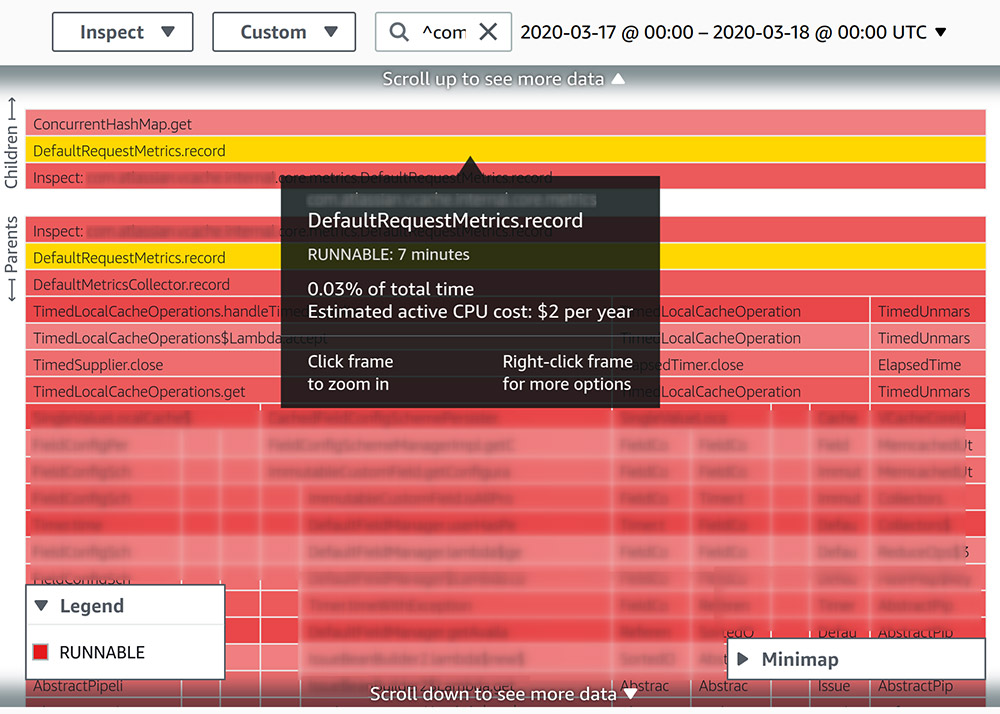
The following screenshot shows a profile of a similar 24-hour period. After we implemented the change, the relevant stack trace is now all in a RUNNABLE state.
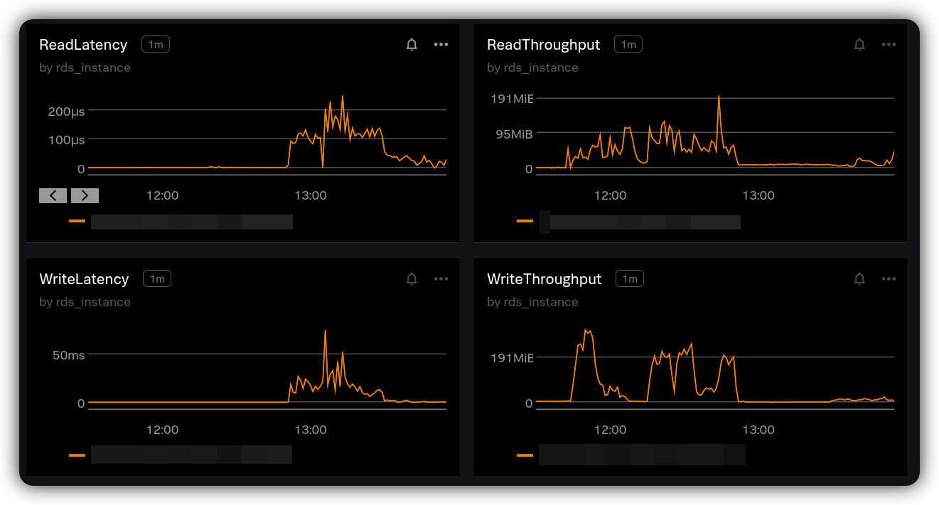
In a more complicated context, AWS CodeGuru Profiler helped to verify how similar code paths in the same stack trace might be performing different operations such as database writes or reads. One of the core metrics that is observed for Jira is the latency of a request and the latency of DB operations per HTTP endpoint. The following shows an observed regression on both request and DB latency on a specific endpoint although the load on the endpoint does not show a change or spike:
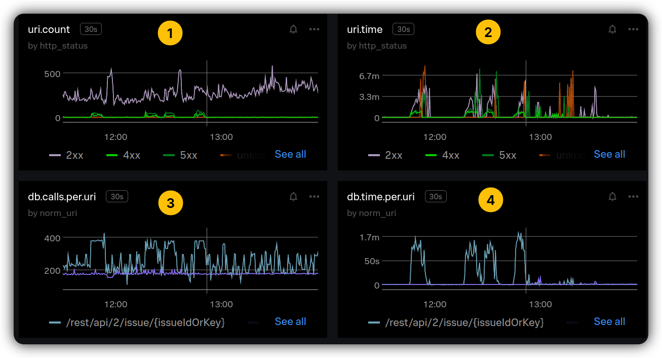
1️⃣ and 2️⃣ show the latency and count for HTTP request while 3️⃣ and 4️⃣ show the latency and count for the database layer for the same HTTP request. Where the spikes occur on 2️⃣ and 4️⃣, we do not observe any noticeable change on 1️⃣ and 3️⃣. How could we explain this?
In our observability stack, we have built another useful tool that captures and maintains a set of metrics mapping HTTP endpoints and SQL statements that are executed. In a simplified version, the following was observed based on the above metrics, that is trying to find the most costly SQL on the HTTP endpoints that has spikes for latency of request and DB:
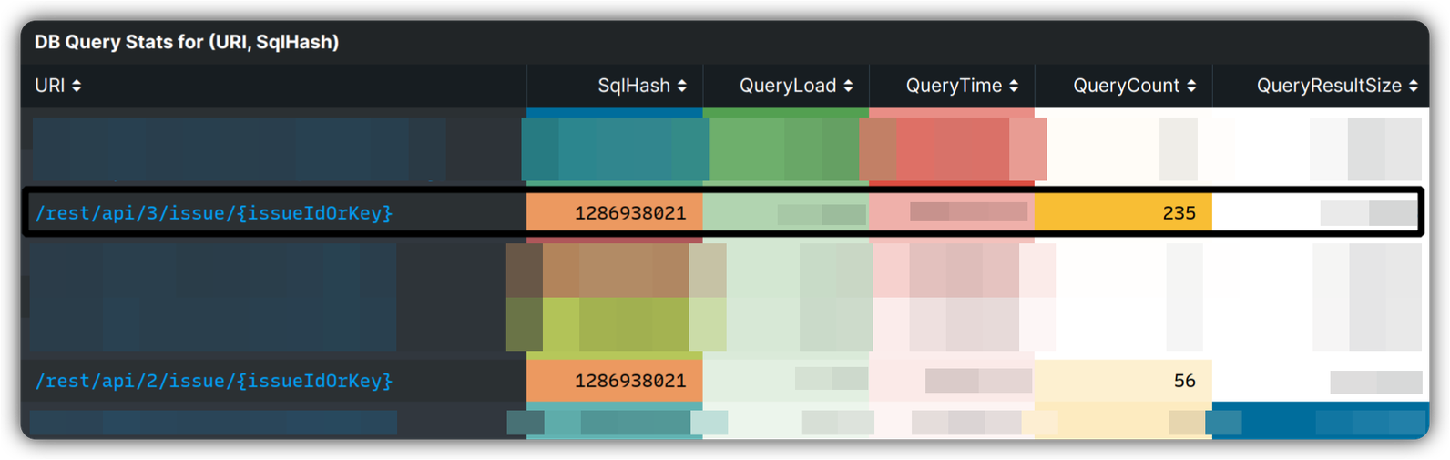
Having the SQL hash, we map it to the class that runs the query. Zooming into the same time window, we observe the following on AWS CodeGuru Profiler for SQL running class. In this case, we search for a class and then use visualization on “latency” per thread states
( = TIMED_WAITING, = WAITING, = RUNNABLE )
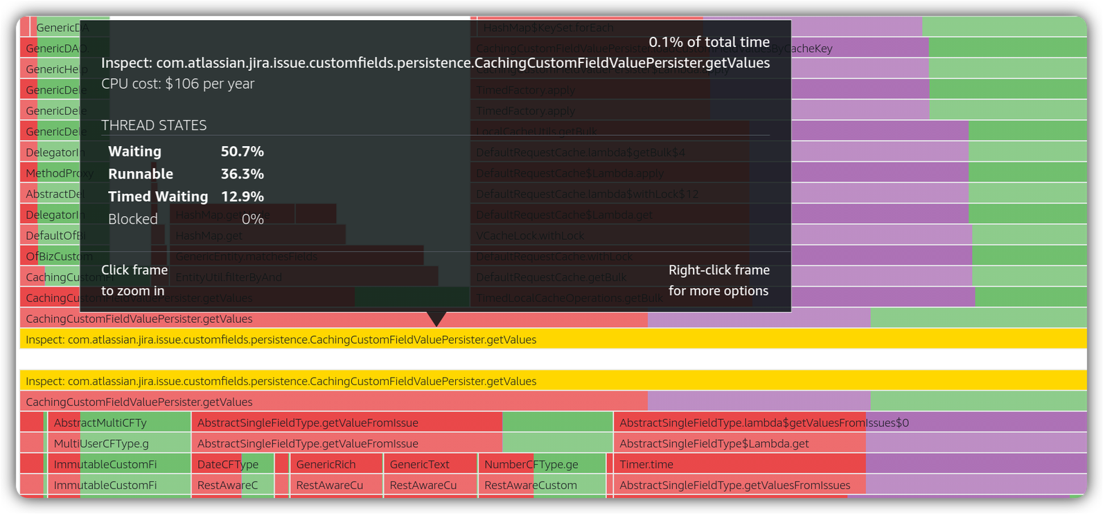
Why is the highlighted class spending it runtime mostly on WAITING and TIMED_WAITING?
One interesting thing is that the proportion of thread states look to be in the same ratio before the stack trace reaches this class at runtime. Therefore, there might be a cause in the stack trace prior to this stack trace element. We move up the stack trace trying to hunt for any interesting observation around issue HTTP endpoints.
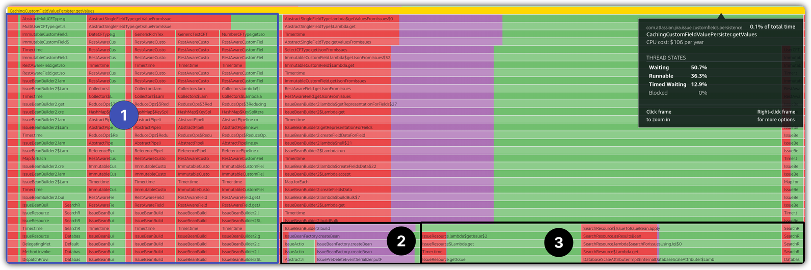
There’re two interesting observations from the above stack trace snapshot:
- 1️⃣ and 3️⃣ subsection of the parent stack trace does not contain any TIMED_WAITING ✅. It’s only 2️⃣ that contains TIMED_WAITING thread state.
- Both operations of write and read seem to be executing in the same stack trace but in different threads.
When we move a bit further up the stack trace on 2️⃣ and 3️⃣ paths:
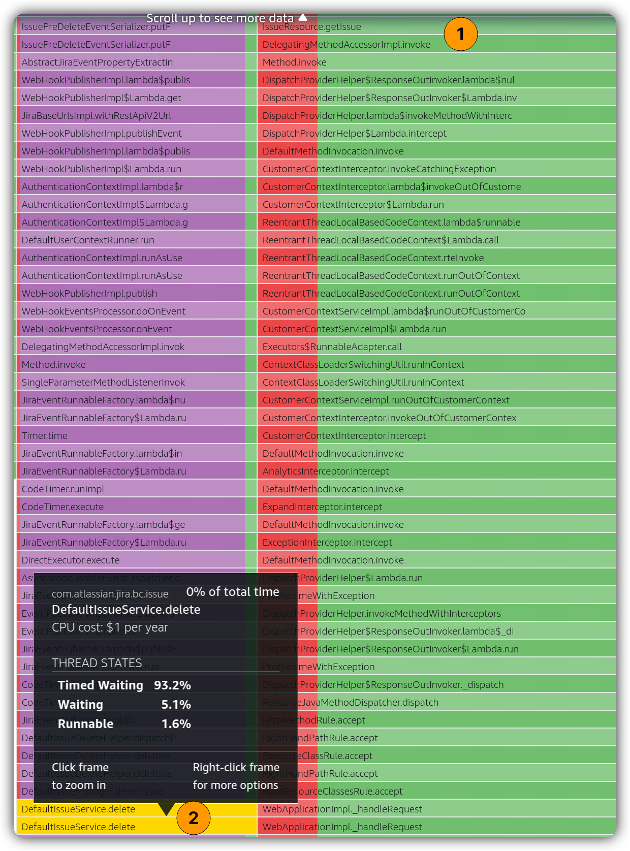
The above observation implies there could be different types of concurrent issue operations at the same time. This was confirmed by looking at database metrics and finding a specific one that shows a matching pattern:
Going back to the starting question to understand the short-timed regression on request and database latency without a change on request load:
A few tenants on Jira started to synchronize their issue data using scheduled jobs and plugins. The operations involved both read and write operations including both HTTP PUT (create issue) and HTTP DELETE (delete issue). To ensure the consistency and integrity of data, there is a locking mechanism applied before deleting an issue which explains TIMED_WAITING — the service was waiting to obtain a lock to be able to delete the issues or create new ones. And, on the other side, there were searches on issue that were receiving issue data which explains WAITING.
✅ In this investigation, in a nutshell:
- We started from our high-level service metrics, such as request latency and database latency.
- We mapped HTTP endpoints to classes and SQL statements that are executed for the endpoint.
- We continued to investigate the relevant classes in Amazon CodeGuru Profiler with the most costly SQL execution.
- In Amazon CodeGuru Profiler, we specifically utilized the “latency” view to observe the proportion of thread states in JVM runtime.
- We explored the stack trace to understand different thread state’s latency to find the first stack trace element causing specific thread states.
- We found that a single stack trace is performing IO operations on database both on read and write mode.
- We verified the database metrics to match the observed thread states.
- We finally found tenant operations and sources of the requests that caused both read and write operations in a short amount of time leading to a saturation and regression of request latency.
⭐️ Bonus Insight:
If you noticed, in the screenshots of Amazon CodeGuru Profiler, the top right corner of a black box shows a very small percentage < 1.0% or ever 0% which is the percentage of the runtime of that stack trace element to the total runtime of the service.
It is fascinating that such a small portion of runtime is able to cause a noticeable regression in request and database latency. In a matter of sub-seconds, the database is saturated with IO operations, and requests are started to be queued up and the latency degrades.
It takes noticeable amounts of effort to perform the investigation, understand the root causes, and then try to improve the products and services. That is something we never hesitate to go through for our customers’ experience.
It has been an amazing journey to evolve our performance engineering tooling. The practice of continuous profiling on JVM applications has shown its great value to many teams across Atlassian. And, the journey continues. In future posts, we will share our experience of tooling when it comes to some of the limitations of Amazon CodeGuru Profiler to capturing native or OS-specific call stacks. In addition, we’re now looking at applying continuous profiling to technology stacks other than JVM. Finally, continuous profiling of JVM applications for memory usage and allocation is one of the next interesting challenges that we’re looking into.
Stay tuned for future stages of our performance engineering journey.